PBR --- IBL Diffuse Irradiance

Introduction

IBL, or image based lighting, is a collection of techniques to light objects, not by direct analytical lights as in the previous chapter, but by treating the surrounding environment as one big light source. This is generally accomplished by manipulating a cubemap environment map (taken from the real world or generated from a 3D scene) such that we can directly use it in our lighting equations: treating each cubemap texel as a light emitter. This way we can effectively capture an environment’s global lighting and general feel, giving objects a better sense of belonging in their environment.

IBL，即基于图像的光照，是一类物体光照技术的集合，它并非像前一章那样直接面对可分析的光源，而是将周围环境视为一个大光源。通常是利用立方体环境贴图（取自真实世界或由 3D 场景生成）来模拟这个大光源，并且可以在光照方程中直接使用该贴图：将立方体贴图每个像素视为一个发光体。这样，我们就能有效捕捉环境的全局光照和总体感觉，让物体更好地融入其所在的环境当中。

As image based lighting algorithms capture the lighting of some (global) environment, its input is considered a more precise form of ambient lighting, even a crude approximation of global illumination. This makes IBL interesting for PBR as objects look significantly more physically accurate when we take the environment’s lighting into account.

由于基于图像的光照算法会捕捉部分（甚至全局）的环境光照，因此其输入被认为是一种更精确的环境光照形式，甚至是全局光照的粗略近似。IBL 会令 PBR 非常有趣，因为当我们将环境光照考虑在内时，物体看起来会带有精确的物理效果。

To start introducing IBL into our PBR system let’s again take a quick look at the reflectance equation:

为了将 IBL 引入 PBR 系统，让我们再次快速浏览一下反射方程：

\[L_o{\small(p,\omega_o)} = \int\limits_{\Omega} \big( k_d\frac{c}{\pi} + k_s\frac{DFG}{4 \big( \omega_o \cdot n \big) \big( \omega_i \cdot n \big)} \big) L_i{\small(p,\omega_i)} \big( n \cdot \omega_i \big) d\omega_i\]

注意：$L_i{\small(p,\omega_i)}$ 是函数，这里面的括号指明函数的参数，表示 $L_i$ 是关于参数 $p$ 和 $\omega_i$ 的函数。而 $\big( n \cdot \omega_i \big)$ 是代数表达式，这里面的括号作用是指明运算优先级，优先进行 $n$ 和 $\omega_i$ 的点积运算。注意认识函数和代数表达式，防止因括号造成混淆误解。$L_i{\small(p,\omega_i)} \big( n \cdot \omega_i \big)$ 是上述二者的数乘。

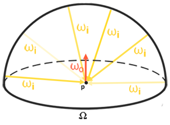
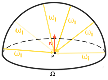
As described before, our main goal is to solve the integral of all incoming light directions $w_i$ over the hemisphere $\Omega$ . Solving the integral in the previous chapter was easy as we knew beforehand the exact few light directions $w_i$ that contributed to the integral. This time however, every incoming light direction $w_i$ from the surrounding environment could potentially have some radiance making it less trivial to solve the integral. This gives us two main requirements for solving the integral:

如前所述，我们的主要目标是求解半球 $\Omega$ 上所有入射光方向 $w_i$ 的积分。上一章中求解该积分较为容易，因为我们事先知道对积分有贡献的确切的几个光照方向 $w_i$。但现在，周围环境中每个入射方向 $w_i$ 上的光照都可能会携带一些辐射，这就使得求解积分变得不那么简单了。求解该积分时我们需要考虑以下两个主要问题：

• We need some way to retrieve the scene’s radiance given any direction vector $w_i$.
• 我们需要一种方法，以便在给定任意方向向量 $w_i$ 时获取场景辐射率。
• Solving the integral needs to be fast and real-time.
• 快速且实时的求解积分。

Now, the first requirement is relatively easy. We’ve already hinted it, but one way of representing an environment or scene’s irradiance is in the form of a (processed) environment cubemap. Given such a cubemap, we can visualize every texel of the cubemap as one single emitting light source. By sampling this cubemap with any direction vector $w_i$, we retrieve the scene’s radiance from that direction.

第一个问题相对简单。我们之前已经有过暗示，表示环境或场景辐照度的一种方法是（经过处理的）环境立方体贴图。有了这样一个立方体贴图，我们就可以将立方体贴图中的每一个像素视作一个发光光源。通过在任一方向向量 $w_i$ 上对立方体贴图进行采样，我们就能获取该方向上场景的辐射率。

Getting the scene’s radiance given any direction vector $w_i$ is then as simple as:

在任一方向向量 $w_i$ 上，获取场景的辐射率非常简单：

vec3 radiance = texture(_cubemapEnvironment, w_i).rgb;

Still, solving the integral requires us to sample the environment map from not just one direction, but all possible directions $w_i$ over the hemisphere $\Omega$ which is far too expensive for each fragment shader invocation. To solve the integral in a more efficient fashion we’ll want to pre-process or pre-compute most of the computations. For this we’ll have to delve a bit deeper into the reflectance equation:

第二个问题就相对复杂了。求解积分要求我们从半球 $\Omega$ 上所有可能的方向 $w_i$ 对环境贴图进行采样，而不只是从某一个方向。对于每次片段着色器调用来说，这样做的开销实在太大了。为了以更高效的方式求解积分，我们需要对大部分计算进行预处理或预计算。为此，我们需要更深入地探究一下反射方程：

\[L_o{\small(p,\omega_o)} = \int\limits_{\Omega} \big( k_d\frac{c}{\pi} + k_s\frac{DFG}{4 \big( \omega_o \cdot n \big) \big( \omega_i \cdot n \big)} \big) L_i{\small(p,\omega_i)} \big(n \cdot \omega_i \big) d\omega_i\]

Taking a good look at the reflectance equation we find that the diffuse $k_d$ and specular $k_s$ term of the BRDF are independent from each other and we can split the integral in two:

仔细观察反射方程，我们会发现双向反射分布函数（BRDF）中的漫反射项 $k_d$ 和镜面反射项 $k_s$ 是相互独立的，这样我们就可以将这个积分拆分成两部分：

\[L_o{\small(p,\omega_o)} = \int\limits_{\Omega} \big( k_d\frac{c}{\pi} \big) L_i{\small(p,\omega_i)} \big(n \cdot \omega_i \big) d\omega_i + \int\limits_{\Omega} \big( k_s\frac{DFG}{4 \big( \omega_o \cdot n \big) \big( \omega_i \cdot n \big) } \big) L_i{\small(p,\omega_i)} \big(n \cdot \omega_i \big) d\omega_i\]

By splitting the integral in two parts we can focus on both the diffuse and specular term individually; the focus of this chapter being on the diffuse integral.

通过将积分拆分成两部分，我们能够分别专注于漫反射项和镜面反射项。本章的重点是漫反射积分。

Taking a closer look at the diffuse integral we find that the diffuse lambert term is a constant term (the color $c$, the refraction ratio $k_d$, and $\pi$ are constant over the integral) and not dependent on any of the integral variables. Given this, we can move the constant term out of the diffuse integral:

进一步仔细观察漫反射积分，我们会发现漫反射兰伯特项是一个常数项（在这个积分中，颜色 $c$、折射比 $k_d$ 以及 $\pi$ 都是常数），并且不依赖于任何积分变量。鉴于此，我们可以把这个常数项从漫反射积分中提取出来：

\[L_o{\small(p,\omega_o)} = k_d\frac{c}{\pi} \int\limits_{\Omega} L_i{\small(p,\omega_i)} \big(n \cdot \omega_i \big) d\omega_i\]

This gives us an integral that only depends on $w_i$ (assuming $p$ is at the center of the environment map). With this knowledge, we can calculate or pre-compute a new cubemap that stores in each sample direction (or texel) $w_o$ the diffuse integral’s result by convolution.

这样我们就得到了一个仅依赖于 $w_i$ 的积分（假设 $p$ 位于环境贴图的中心）。基于这一认识，我们可以通过卷积来计算或预计算一个新的立方体贴图，在该立方体贴图每个采样方向 $w_o$ 上的纹素中存储漫反射积分的结果。

Convolution is applying some computation to each entry in a data set considering all other entries in the data set; the data set being the scene’s radiance or environment map. Thus for every sample direction in the cubemap, we take all other sample directions over the hemisphere $\Omega$ into account.

卷积是在综合考虑数据集中其他条目的情况下，对每个条目进行特定计算的操作。在这里，数据集就是场景的辐射率或者环境贴图。因此，对于立方体贴图中的每个采样方向，我们会将半球面 $\Omega$ 上的所有其他采样方向都考虑在内。

To convolute an environment map we solve the integral for each output $w_o$ sample direction by discretely sampling a large number of directions $w_i$ over the hemisphere $\Omega$ and averaging their radiance. The hemisphere we build the sample directions $w_i$ from is oriented towards the output $w_o$ sample direction we’re convoluting.

为了对环境贴图进行卷积操作，我们对半球面 $\Omega$ 上大量的方向 $w_i$ 进行离散采样，并求这些方向的辐射率平均值，从而求解每个输出采样方向 $w_o$ 的积分。我们用来建立输入采样方向 $w_i$ 的半球，其朝向是我们正在进行卷积计算的输出采样方向 $w_o$。

This pre-computed cubemap, that for each sample direction $w_o$ stores the integral result, can be thought of as the pre-computed sum of all indirect diffuse light of the scene hitting some surface aligned along direction $w_o$. Such a cubemap is known as an irradiance map seeing as the convoluted cubemap effectively allows us to directly sample the scene’s (pre-computed) irradiance from any direction $w_o$.

这个预计算的立方体贴图为每个输出采样方向 $w_o$ 存储了积分结果，可以理解为：它预先计算了场景中所有照射到表面点 $p$ 的间接漫反射光沿出射方向 $w_o$ 反射的总量。这种立方体贴图被称为辐照度图（irradiance map），因为经过卷积处理的立方体贴图让我们能够直接从任意方向 $w_o$ 采样场景的（预先计算的）辐照度。

The radiance equation also depends on a position $p$, which we’ve assumed to be at the center of the irradiance map. This does mean all diffuse indirect light must come from a single environment map which may break the illusion of reality (especially indoors). Render engines solve this by placing reflection probes all over the scene where each reflection probes calculates its own irradiance map of its surroundings. This way, the irradiance (and radiance) at position $p$ is the interpolated irradiance between its closest reflection probes. For now, we assume we always sample the environment map from its center.

辐射度方程还依赖于位置 $p$（我们之前默认该位置位于辐照度图的中心）。这意味着所有漫反射间接光必然都来自单一环境贴图，这可能会破坏真实感（尤其在室内场景中）。渲染引擎解决这个问题的方案是在场景中布置反射探针，每个探针会计算它自己周围的辐照度图。通过这种方式，位置 $p$ 处的辐照度（及辐射率）由其最近反射探针的插值结果决定。当前我们暂定总是从环境贴图中心进行采样。

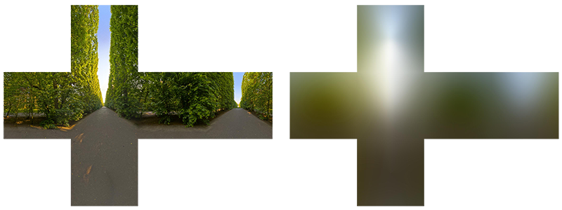
Below is an example of a cubemap environment map and its resulting irradiance map (courtesy of wave engine), averaging the scene’s radiance for every direction $w_o$.

下图示例展示了一个立方体环境贴图及其生成的辐照度图（由 Wave Engine 提供），该图通过对场景中每个方向 $w_o$ 的辐射率进行平均计算得出。

By storing the convoluted result in each cubemap texel (in the direction of $w_o$), the irradiance map displays somewhat like an average color or lighting display of the environment. Sampling any direction from this environment map will give us the scene’s irradiance in that particular direction.

通过将卷积结果存储在每个立方体贴图的纹素中（对应方向 $w_o$），辐照度图会呈现出类似环境平均颜色/光照的效果。从该贴图中采样任意方向，即可获得场景在该特定方向上的辐照度数据。

PBR and HDR

We’ve briefly touched upon it in the previous chapter: taking the high dynamic range of your scene’s lighting into account in a PBR pipeline is incredibly important. As PBR bases most of its inputs on real physical properties and measurements it makes sense to closely match the incoming light values to their physical equivalents. Whether we make educated guesses on each light’s radiant flux or use their direct physical equivalent, the difference between a simple light bulb or the sun is significant either way. Without working in an HDR render environment it’s impossible to correctly specify each light’s relative intensity.

我们在前一章节中曾简要提及：在 PBR（基于物理的渲染）管线中，把场景光照的高动态范围（HDR）特性考虑在内至关重要。由于 PBR 流程的大部分输入参数都基于真实物理属性和测量数据，因此使入射光的值尽可能接近其物理等效值就显得十分必要。例如无论是估算还是物理实测，普通灯泡与太阳的光照强度差异都极为显著。若未采用 HDR 渲染环境，将无法准确界定各光源的相对强度。

So, PBR and HDR go hand in hand, but how does it all relate to image based lighting? We’ve seen in the previous chapter that it’s relatively easy to get PBR working in HDR. However, seeing as for image based lighting we base the environment’s indirect light intensity on the color values of an environment cubemap we need some way to store the lighting’s high dynamic range into an environment map.

因此，PBR 与 HDR 技术必须配合使用，但是这与基于图像的照明又有何关联？我们在前一章节已经证实，在 HDR 环境下实现 PBR 相对简单。但考虑到 IBL 需要根据立方体环境贴图的颜色值来确定环境中的间接光强度，就必须找到将 HDR 光照数据存储到环境贴图中的方法。

The environment maps we’ve been using so far as cubemaps (used as skyboxes for instance) are in low dynamic range (LDR). We directly used their color values from the individual face images, ranged between 0.0 and 1.0, and processed them as is. While this may work fine for visual output, when taking them as physical input parameters it’s not going to work.

我们之前使用的立方体贴图（例如作为天空盒的贴图）都是低动态范围（LDR）的。是直接使用各个面的图像颜色值（在 0.0 到 1.0 范围内）并对它们进行处理。虽然这种处理对于视觉输出尚可接受，但若将其作为物理输入参数则完全不可行。

The radiance HDR file format

Enter the radiance file format. The radiance file format (with the .hdr extension) stores a full cubemap with all 6 faces as floating point data. This allows us to specify color values outside the 0.0 to 1.0 range to give lights their correct color intensities. The file format also uses a clever trick to store each floating point value, not as a 32 bit value per channel, but 8 bits per channel using the color’s alpha channel as an exponent (this does come with a loss of precision). This works quite well, but requires the parsing program to re-convert each color to their floating point equivalent.

在此引入辐射率文件格式。这种以 .hdr 为扩展名的文件格式，将包含 6 个面的完整的立方体贴图以浮点数据形式存储，使我们能够指定超出 0.0 到 1.0 范围的颜色值，从而准确表达光源的真实强度。这种文件格式也采用了一种独特技巧去存储每个浮点值，即不是为每个通道使用 32 位值，而是每个通道使用 8 位，并将颜色的 alpha 通道用作指数（这会带来一定的精度损失）。这种方法效果相当不错，但需要解析程序将每种颜色重新转换为对应的浮点值。

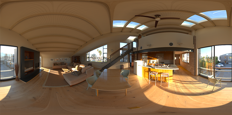
There are quite a few radiance HDR environment maps freely available from sources like sIBL archive of which you can see an example below:

有相当多的辐射率 HDR 环境贴图可以从像 sIBL 这样的资源库中免费获取，下面你可以看到一个例子：

This may not be exactly what you were expecting, as the image appears distorted and doesn’t show any of the 6 individual cubemap faces of environment maps we’ve seen before. This environment map is projected from a sphere onto a flat plane such that we can more easily store the environment into a single image known as an equirectangular map. This does come with a small caveat as most of the visual resolution is stored in the horizontal view direction, while less is preserved in the bottom and top directions. In most cases this is a decent compromise as with almost any renderer you’ll find most of the interesting lighting and surroundings in the horizontal viewing directions.

这可能和你预想的不太一样，因为这张图像看起来有畸变，而且也没有展示出我们之前见过的环境贴图的 6 个独立立方体面。这种环境贴图是从球体投影到一个平面上的，这样我们就能更轻松地将整个环境信息存储在一张被称为等距柱状投影图（全景图）的图像里。不过这里有个小问题，大部分视觉分辨率集中在水平视角方向，而顶部和底部方向保留的分辨率较低。但在大多数情况下，这是个不错的折中方案，因为在几乎所有渲染器中，你会发现水平视角方向有最值得关注的光照和周边环境信息。

HDR and stb_image.h

Loading radiance HDR images directly requires some knowledge of the file format which isn’t too difficult, but cumbersome nonetheless. Lucky for us, the popular one header library stb_image.h supports loading radiance HDR images directly as an array of floating point values which perfectly fits our needs. With stb_image added to your project, loading an HDR image is now as simple as follows:

直接加载辐射率 HDR 图像需要对其文件格式有一定了解，这倒不算太难，但总归还是有些繁琐。好在，知名的单头文件库 stb_image.h 支持直接将辐射率 HDR 图像加载为浮点数值数组，这正合我们的需求。将 stb_image 添加到你的项目后，加载 HDR 图像就变得十分简单，如下所示：

#include "stb_image.h"
[...]

stbi_set_flip_vertically_on_load(true);
int width, height, nrComponents;
float *data = stbi_loadf("newport_loft.hdr", &width, &height, &nrComponents, 0);
unsigned int hdrTexture;
if (data)
{
    glGenTextures(1, &hdrTexture);
    glBindTexture(GL_TEXTURE_2D, hdrTexture);
    glTexImage2D(GL_TEXTURE_2D, 0, GL_RGB16F, width, height, 0, GL_RGB, GL_FLOAT, data); 

    glTexParameteri(GL_TEXTURE_2D, GL_TEXTURE_WRAP_S, GL_CLAMP_TO_EDGE);
    glTexParameteri(GL_TEXTURE_2D, GL_TEXTURE_WRAP_T, GL_CLAMP_TO_EDGE);
    glTexParameteri(GL_TEXTURE_2D, GL_TEXTURE_MIN_FILTER, GL_LINEAR);
    glTexParameteri(GL_TEXTURE_2D, GL_TEXTURE_MAG_FILTER, GL_LINEAR);

    stbi_image_free(data);
}
else
{
    std::cout << "Failed to load HDR image." << std::endl;
}  

stb_image.h automatically maps the HDR values to a list of floating point values: 32 bits per channel and 3 channels per color by default. This is all we need to store the equirectangular HDR environment map into a 2D floating point texture.

stb_image.h 会自动将 HDR 值映射为一个浮点值列表：默认情况下，每个通道为 32 位，每种颜色有 3 个通道。我们只需利用这些数据，就能将等距柱状投影的 HDR 环境贴图存储为一个二维浮点纹理。

From Equirectangular to Cubemap

It is possible to use the equirectangular map directly for environment lookups, but these operations can be relatively expensive in which case a direct cubemap sample is more performant. Therefore, in this chapter we’ll first convert the equirectangular image to a cubemap for further processing. Note that in the process we also show how to sample an equirectangular map as if it was a 3D environment map in which case you’re free to pick whichever solution you prefer.

可以直接使用等距柱状投影图进行环境查询，但这类操作的开销可能较高，相比之下直接采样立方体贴图的性能更优。因此在本章中，我们会先将等距柱状投影图像转换为立方体贴图，以便进一步处理。需要注意的是，在这个过程中我们还会展示如何将等距柱状投影图当作 3D 环境图进行采样，这样你就可以自由选择更适合的方案。

To convert an equirectangular image into a cubemap we need to render a (unit) cube and project the equirectangular map on all of the cube’s faces from the inside and take 6 images of each of the cube’s sides as a cubemap face. The vertex shader of this cube simply renders the cube as is and passes its local position to the fragment shader as a 3D sample vector:

要将等距柱状投影图像转换为立方体贴图，我们需要渲染一个（单位）立方体，并从内部将等距柱状投影图投射到立方体的所有面上，然后将立方体每个面的图像分别作为立方体贴图的一个面保存下来。这个立方体的顶点着色器仅负责按原样渲染立方体，并将其局部位置作为 3D 采样向量传递给片段着色器：

#version 330 core
layout (location = 0) in vec3 aPos;

out vec3 localPos;

uniform mat4 projection;
uniform mat4 view;

void main()
{
    localPos = aPos;  
    gl_Position =  projection * view * vec4(localPos, 1.0);
}

For the fragment shader, we color each part of the cube as if we neatly folded the equirectangular map onto each side of the cube. To accomplish this, we take the fragment’s sample direction as interpolated from the cube’s local position and then use this direction vector and some trigonometry magic (spherical to cartesian) to sample the equirectangular map as if it’s a cubemap itself. We directly store the result onto the cube-face’s fragment which should be all we need to do:

对于片段着色器，我们要为立方体的每个部分着色，就好像把等距柱状投影图完美地贴合到立方体的每个面上。为实现这一点，我们先根据立方体的局部位置进行插值，得到片段的采样方向。接着，利用这个方向向量，结合一些三角学知识（从球面坐标转换为笛卡尔坐标），将等距柱状投影图当作立方体贴图来采样。最后，我们把采样结果直接存储到立方体表面的片段中，这样就大功告成了。

#version 330 core
out vec4 FragColor;
in vec3 localPos;

uniform sampler2D equirectangularMap;

const vec2 invAtan = vec2(0.1591, 0.3183);
vec2 SampleSphericalMap(vec3 v)
{
    vec2 uv = vec2(atan(v.z, v.x), asin(v.y));
    uv *= invAtan;
    uv += 0.5;
    return uv;
}

void main()
{		
    vec2 uv = SampleSphericalMap(normalize(localPos)); // make sure to normalize localPos
    vec3 color = texture(equirectangularMap, uv).rgb;
    
    FragColor = vec4(color, 1.0);
}

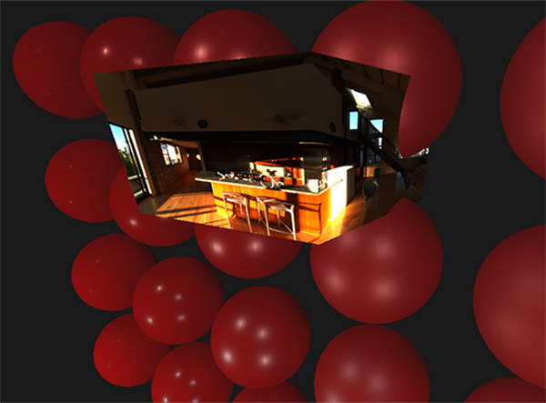
If you render a cube at the center of the scene given an HDR equirectangular map you’ll get something that looks like this:

如果在场景中心渲染一个立方体，并为其应用 HDR 等距柱状投影图，你会得到类似这样的效果：

This demonstrates that we effectively mapped an equirectangular image onto a cubic shape, but doesn’t yet help us in converting the source HDR image to a cubemap texture. To accomplish this we have to render the same cube 6 times, looking at each individual face of the cube, while recording its visual result with a framebuffer object:

这表明我们已成功将等距柱状投影图像映射到了立方体形状上，但这还不足以帮助我们将源 HDR 图像转换为立方体贴图纹理。为实现这一点，我们必须将同一个立方体渲染 6 次，每次分别看向立方体的一个面，同时使用一个帧缓冲对象记录其可视化后的结果：

unsigned int captureFBO, captureRBO;
glGenFramebuffers(1, &captureFBO);
glGenRenderbuffers(1, &captureRBO);

glBindFramebuffer(GL_FRAMEBUFFER, captureFBO);
glBindRenderbuffer(GL_RENDERBUFFER, captureRBO);
glRenderbufferStorage(GL_RENDERBUFFER, GL_DEPTH_COMPONENT24, 512, 512);
glFramebufferRenderbuffer(GL_FRAMEBUFFER, GL_DEPTH_ATTACHMENT, GL_RENDERBUFFER, captureRBO);

Of course, we then also generate the corresponding cubemap color textures, pre-allocating memory for each of its 6 faces:

当然，我们随后还要生成相应的立方体贴图颜色纹理，并为其 6 个面中的每一个预先分配内存：

unsigned int envCubemap;
glGenTextures(1, &envCubemap);
glBindTexture(GL_TEXTURE_CUBE_MAP, envCubemap);
for (unsigned int i = 0; i < 6; ++i)
{
    // note that we store each face with 16 bit floating point values
    glTexImage2D(GL_TEXTURE_CUBE_MAP_POSITIVE_X + i, 0, GL_RGB16F, 
                 512, 512, 0, GL_RGB, GL_FLOAT, nullptr);
}
glTexParameteri(GL_TEXTURE_CUBE_MAP, GL_TEXTURE_WRAP_S, GL_CLAMP_TO_EDGE);
glTexParameteri(GL_TEXTURE_CUBE_MAP, GL_TEXTURE_WRAP_T, GL_CLAMP_TO_EDGE);
glTexParameteri(GL_TEXTURE_CUBE_MAP, GL_TEXTURE_WRAP_R, GL_CLAMP_TO_EDGE);
glTexParameteri(GL_TEXTURE_CUBE_MAP, GL_TEXTURE_MIN_FILTER, GL_LINEAR);
glTexParameteri(GL_TEXTURE_CUBE_MAP, GL_TEXTURE_MAG_FILTER, GL_LINEAR);

Then what’s left to do is capture the equirectangular 2D texture onto the cubemap faces.

接下来要做的就是把等距柱状投影的二维纹理映射到立方体贴图的各个面上。

I won’t go over the details as the code details topics previously discussed in the framebuffer and point shadows chapters, but it effectively boils down to setting up 6 different view matrices (facing each side of the cube), set up a projection matrix with a fov of 90 degrees to capture the entire face, and render a cube 6 times storing the results in a floating point framebuffer:

我就不详细展开了，因为代码细节涉及之前在帧缓冲和点光源阴影章节中讨论过的内容。但实际上，主要步骤就是设置 6 个不同的视图矩阵（分别朝向立方体的每个面），设置一个视野为 90 度的投影矩阵以捕获整个面，然后将立方体渲染 6 次，并把结果存储在一个浮点型帧缓冲中。

glm::mat4 captureProjection = glm::perspective(glm::radians(90.0f), 1.0f, 0.1f, 10.0f);
glm::mat4 captureViews[] = 
{
   glm::lookAt(glm::vec3(0.0f, 0.0f, 0.0f), glm::vec3( 1.0f,  0.0f,  0.0f), glm::vec3(0.0f, -1.0f,  0.0f)),
   glm::lookAt(glm::vec3(0.0f, 0.0f, 0.0f), glm::vec3(-1.0f,  0.0f,  0.0f), glm::vec3(0.0f, -1.0f,  0.0f)),
   glm::lookAt(glm::vec3(0.0f, 0.0f, 0.0f), glm::vec3( 0.0f,  1.0f,  0.0f), glm::vec3(0.0f,  0.0f,  1.0f)),
   glm::lookAt(glm::vec3(0.0f, 0.0f, 0.0f), glm::vec3( 0.0f, -1.0f,  0.0f), glm::vec3(0.0f,  0.0f, -1.0f)),
   glm::lookAt(glm::vec3(0.0f, 0.0f, 0.0f), glm::vec3( 0.0f,  0.0f,  1.0f), glm::vec3(0.0f, -1.0f,  0.0f)),
   glm::lookAt(glm::vec3(0.0f, 0.0f, 0.0f), glm::vec3( 0.0f,  0.0f, -1.0f), glm::vec3(0.0f, -1.0f,  0.0f))
};

// convert HDR equirectangular environment map to cubemap equivalent
equirectangularToCubemapShader.use();
equirectangularToCubemapShader.setInt("equirectangularMap", 0);
equirectangularToCubemapShader.setMat4("projection", captureProjection);
glActiveTexture(GL_TEXTURE0);
glBindTexture(GL_TEXTURE_2D, hdrTexture);

glViewport(0, 0, 512, 512); // don't forget to configure the viewport to the capture dimensions.
glBindFramebuffer(GL_FRAMEBUFFER, captureFBO);
for (unsigned int i = 0; i < 6; ++i)
{
    equirectangularToCubemapShader.setMat4("view", captureViews[i]);
    glFramebufferTexture2D(GL_FRAMEBUFFER, GL_COLOR_ATTACHMENT0, 
                           GL_TEXTURE_CUBE_MAP_POSITIVE_X + i, envCubemap, 0);
    glClear(GL_COLOR_BUFFER_BIT | GL_DEPTH_BUFFER_BIT);

    renderCube(); // renders a 1x1 cube
}
glBindFramebuffer(GL_FRAMEBUFFER, 0);  

We take the color attachment of the framebuffer and switch its texture target around for every face of the cubemap, directly rendering the scene into one of the cubemap’s faces. Once this routine has finished (which we only have to do once), the cubemap envCubemap should be the cubemapped environment version of our original HDR image.

我们获取帧缓冲的颜色附件，并针对立方体贴图的每个面切换其纹理目标，将场景直接渲染到立方体贴图的其中一个面上。一旦这个流程完成（我们只需执行一次），立方体贴图 envCubemap 就应该是我们原始 HDR 图像的立方体贴图形式的环境版本了。

Let’s test the cubemap by writing a very simple skybox shader to display the cubemap around us:

让我们编写一个非常简单的天空盒着色器来显示环绕我们的立方体贴图，以此来测试这个立方体贴图：

#version 330 core
layout (location = 0) in vec3 aPos;

uniform mat4 projection;
uniform mat4 view;

out vec3 localPos;

void main()
{
    localPos = aPos;

    mat4 rotView = mat4(mat3(view)); // remove translation from the view matrix
    vec4 clipPos = projection * rotView * vec4(localPos, 1.0);

    gl_Position = clipPos.xyww;
}

Note the xyww trick here that ensures the depth value of the rendered cube fragments always end up at 1.0, the maximum depth value, as described in the cubemap chapter. Do note that we need to change the depth comparison function to GL_LEQUAL:

注意这里使用了 xyww 技巧，正如立方体贴图章节所描述的，这能确保渲染的立方体片段的深度值始终为 1.0，也就是最大深度值。要注意，我们需要将深度比较函数更改为 GL_LEQUAL。

在 OpenGL 中，深度测试用于确定哪些片段应该被绘制，哪些应该被丢弃。默认的深度比较函数可能是 GL_LESS，即如果新片段的深度值小于当前深度缓冲区中的值，那么新片段会被绘制。而使用 xyww 技巧后，我们希望当新片段的深度值小于或等于当前深度缓冲区中的值时就绘制，所以要把深度比较函数改为 GL_LEQUAL。

glDepthFunc(GL_LEQUAL);

The fragment shader then directly samples the cubemap environment map using the cube’s local fragment position:

片段着色器随后直接使用立方体的局部片段位置对立方体贴图环境贴图进行采样：

#version 330 core
out vec4 FragColor;

in vec3 localPos;
  
uniform samplerCube environmentMap;
  
void main()
{
    vec3 envColor = texture(environmentMap, localPos).rgb;
    
    envColor = envColor / (envColor + vec3(1.0));
    envColor = pow(envColor, vec3(1.0/2.2)); 
  
    FragColor = vec4(envColor, 1.0);
}

We sample the environment map using its interpolated vertex cube positions that directly correspond to the correct direction vector to sample. Seeing as the camera’s translation components are ignored, rendering this shader over a cube should give you the environment map as a non-moving background. Also, as we directly output the environment map’s HDR values to the default LDR framebuffer, we want to properly tone map the color values. Furthermore, almost all HDR maps are in linear color space by default so we need to apply gamma correction before writing to the default framebuffer.

我们使用经过插值处理的立方体顶点位置对环境贴图进行采样，这些位置直接对应着正确的采样方向向量。由于相机的平移分量被忽略了，在一个立方体上应用这个着色器进行渲染，会让你得到一个像静止背景一样的环境贴图。此外，由于我们直接将环境贴图的高动态范围（HDR）值输出到默认的低动态范围（LDR）帧缓冲中，所以需要对颜色值进行适当的色调映射。而且，几乎所有的 HDR 贴图默认都处于线性颜色空间，因此在写入默认帧缓冲之前，我们需要应用伽马校正。

Now rendering the sampled environment map over the previously rendered spheres should look something like this:

现在，将采样得到的环境贴图渲染到之前已渲染好的球体上，呈现出的效果大致如下：

Well… it took us quite a bit of setup to get here, but we successfully managed to read an HDR environment map, convert it from its equirectangular mapping to a cubemap, and render the HDR cubemap into the scene as a skybox. Furthermore, we set up a small system to render onto all 6 faces of a cubemap, which we’ll need again when convoluting the environment map. You can find the source code of the entire conversion process here.

嗯……为了达成这一步，我们做了不少前期准备工作。不过现在，我们已成功读取了一张 HDR 环境贴图，将其从等距柱状投影图转换为了立方体贴图，还把这个 HDR 立方体贴图作为天空盒渲染到了场景中。此外，我们搭建了一个小型系统，可将图像渲染到立方体贴图的所有 6 个面上，在对环境贴图进行卷积操作时，我们还会用到这个系统。你可以在此处找到整个转换过程的源代码。

Cubemap convolution

As described at the start of the chapter, our main goal is to solve the integral for all diffuse indirect lighting given the scene’s irradiance in the form of a cubemap environment map. We know that we can get the radiance of the scene $L(p, w_i)$ in a particular direction by sampling an HDR environment map in direction $w_i$. To solve the integral, we have to sample the scene’s radiance from all possible directions within the hemisphere $\Omega$ for each fragment.

正如本章开头所述，我们的主要目标是：基于立方体贴图环境映射形式的辐照度，求解场景中所有漫反射间接光照的积分。我们知道，通过在特定方向 $w_i$ 上对 HDR 环境贴图进行采样，就能得到场景在该方向上的辐射率 $L(p, w_i)$。为了求解这个积分，我们必须针对每个片段，在半球面 $\Omega$ 内的所有可能方向上对场景的辐射率进行采样。

It is however computationally impossible to sample the environment’s lighting from every possible direction in $\Omega$, the number of possible directions is theoretically infinite. We can however, approximate the number of directions by taking a finite number of directions or samples, spaced uniformly or taken randomly from within the hemisphere, to get a fairly accurate approximation of the irradiance; effectively solving the integral $\int$ discretely.

然而，要从半球面 $\Omega$ 内的每一个可能方向对环境光照进行采样，在计算上是不可能的，因为理论上可能的方向数量是无穷无尽的。不过，我们可以通过选取有限数量的方向或样本（这些样本可以在半球面内均匀分布，也可以随机选取）来近似表示可能的方向数量，从而得到一个相对准确的辐照度近似值；实际上就是对积分 $\int$ 进行离散求解。

It is however still too expensive to do this for every fragment in real-time as the number of samples needs to be significantly large for decent results, so we want to pre-compute this. Since the orientation of the hemisphere decides where we capture the irradiance, we can pre-calculate the irradiance for every possible hemisphere orientation oriented around all outgoing directions $w_o$:

然而，对于每个片段实时进行这样的计算成本仍然过高，因为要想得到不错的结果，所需的样本数量必须相当大。所以，我们希望进行预计算。由于半球的朝向决定了捕获辐照度的位置，我们可以可以围绕所有出射方向 $w_o$，预先计算每个可能的半球朝向对应的辐照度。

\[L_o{\small(p,\omega_o)} = k_d\frac{c}{\pi} \int\limits_{\Omega} L_i{\small(p,\omega_i)} \big(n \cdot \omega_i \big) d\omega_i\]

Given any direction vector $w_i$ in the lighting pass, we can then sample the pre-computed irradiance map to retrieve the total diffuse irradiance from direction $w_i$. To determine the amount of indirect diffuse (irradiant) light at a fragment surface, we retrieve the total irradiance from the hemisphere oriented around its surface normal. Obtaining the scene’s irradiance is then as simple as:

在光照计算阶段，给定任意的方向向量 $w_i$，我们可以对预计算的辐照度图进行采样，从而获取 $w_i$ 方向上总的漫反射辐照度。为了确定某个片段表面的间接漫反射光（辐照度）的总量，我们会围绕该表面法线获取半球内总的辐照度。那么，获取场景的辐照度就变得十分简单，具体如下：

vec3 irradiance = texture(irradianceMap, N).rgb;

Now, to generate the irradiance map, we need to convolute the environment’s lighting as converted to a cubemap. Given that for each fragment the surface’s hemisphere is oriented along the normal vector $N$, convoluting a cubemap equals calculating the total averaged radiance of each direction $w_i$ in the hemisphere $\Omega$ oriented along $N$.

现在，为了生成辐照度图，我们需要对转换为立方体贴图的环境光照进行卷积操作。鉴于每个片段其表面的半球是朝向法线向量 $N$ 的，对立方体贴图进行卷积就等同于在半球 $\Omega$ 内沿着法线向量 $N$ 计算每个方向 $w_i$ 的总平均辐射率。

Thankfully, all of the cumbersome setup of this chapter isn’t all for nothing as we can now directly take the converted cubemap, convolute it in a fragment shader, and capture its result in a new cubemap using a framebuffer that renders to all 6 face directions. As we’ve already set this up for converting the equirectangular environment map to a cubemap, we can take the exact same approach but use a different fragment shader:

所幸，本章中所有繁琐的准备工作并非徒劳。现在，我们可以直接取用转换好的立方体贴图，在片段着色器里对其进行卷积操作，然后借助一个能向所有 6 个面方向渲染的帧缓冲，将结果捕获到一个新的立方体贴图中。由于我们在之前已经搭建好了把等距柱状投影环境图转换为立方体贴图的流程，所以现在可以复用它，只不过要使用一个不同的片段着色器。

#version 330 core
out vec4 FragColor;
in vec3 localPos;

uniform samplerCube environmentMap;

const float PI = 3.14159265359;

void main()
{		
    // the sample direction equals the hemisphere's orientation 
    vec3 normal = normalize(localPos);
  
    vec3 irradiance = vec3(0.0);
  
    [...] // convolution code
  
    FragColor = vec4(irradiance, 1.0);
}

With environmentMap being the HDR cubemap as converted from the equirectangular HDR environment map.

这里的 environmentMap 是 HDR 立方体贴图，从等距柱状投影 HDR 环境贴图转换而来。

There are many ways to convolute the environment map, but for this chapter we’re going to generate a fixed amount of sample vectors for each cubemap texel along a hemisphere $\Omega$ oriented around the sample direction and average the results. The fixed amount of sample vectors will be uniformly spread inside the hemisphere. Note that an integral is a continuous function and discretely sampling its function given a fixed amount of sample vectors will be an approximation. The more sample vectors we use, the better we approximate the integral.

对环境贴图进行卷积的方法有很多，但在本章中，我们将沿着朝向采样方向的半球 $\Omega$，为立方体贴图的每个纹素生成固定数量的采样向量，并对结果求平均。这些固定数量的采样向量会在半球内均匀分布。需要注意的是，积分是一个连续函数，使用固定数量的采样向量对其函数进行离散采样只是一种近似——采样向量越多，对积分的近似效果就越好。

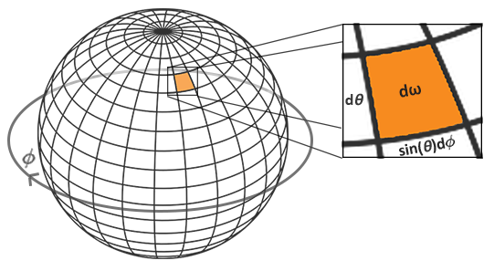
The integral $\int$ of the reflectance equation revolves around the solid angle $dw$ which is rather difficult to work with. Instead of integrating over the solid angle $dw$ we’ll integrate over its equivalent spherical coordinates $\theta$ and $\phi$.

反射方程中的积分 $\int$ 围绕立体角 $d\omega$ 展开，而直接处理立体角较为困难。因此，我们不直接对立体角 $d\omega$ 积分，而是对与之等价的球面坐标 $\theta$（极角）和 $\phi$（方位角）进行积分。

We use the polar azimuth $\phi$ angle to sample around the ring of the hemisphere between $0$ and $2\pi$, and use the inclination zenith $\theta$ angle between $0$ and $\frac{1}{2}\pi$ to sample the increasing rings of the hemisphere. This will give us the updated reflectance integral:

我们使用极方位角 $\phi$ 在 $0$ 到 $2\pi$ 之间沿半球的环向进行采样，并使用天顶倾角 $\theta$ 在 $0$ 到 $\frac{1}{2}\pi$ 之间对半球上半径递增的环进行采样。这将提供给我们更新后的反射积分：

\[L_o{\small(p,\phi_o, \theta_o)} = k_d\frac{c}{\pi} \int_{\phi = 0}^{2\pi} \int_{\theta = 0}^{\frac{1}{2}\pi} L_i{\small(p,\phi_i, \theta_i)} \cos{\small(\theta)} \sin{\small(\theta)} d\phi d\theta\]

Solving the integral requires us to take a fixed number of discrete samples within the hemisphere $\Omega$ and averaging their results. This translates the integral to the following discrete version as based on the Riemann sum given $n1$ and $n2$ discrete samples on each spherical coordinate respectively:

求解这个积分需要我们在半球面 $\Omega$ 内采集一定数量的离散样本，然后对结果求平均值。基于黎曼和，在球面坐标每个维度上分别采样 $n_1$ 和 $n_2$ 个离散样本后，这个积分可以转化为下面的离散形式：

\[L_o{\small(p,\phi_o, \theta_o)} = k_d \frac{c\pi}{n1 n2} \sum_{\phi = 0}^{n1} \sum_{\theta = 0}^{n2} L_i{\small(p,\phi_i, \theta_i)} \cos{\small(\theta)} \sin{\small(\theta)} d\phi d\theta\]

As we sample both spherical values discretely, each sample will approximate or average an area on the hemisphere as the image before shows. Note that (due to the general properties of a spherical shape) the hemisphere’s discrete sample area gets smaller the higher the zenith angle $\theta$ as the sample regions converge towards the center top. To compensate for the smaller areas, we weigh its contribution by scaling the area by $\sin \theta$.

由于我们对球面坐标进行离散采样，每个样本将近似代表半球表面上的一个微小区域，如前图所示。需要注意的是（由于球面的几何特性），天顶角 $\theta$ 越大，半球的离散采样区域面积越小 ——— 因为采样区域在向顶部中心汇聚。为了补偿这种面积变化带来的影响，我们通过将面积乘以 $\sin \theta$ 来对其贡献度做加权处理。

Discretely sampling the hemisphere given the integral’s spherical coordinates translates to the following fragment code:

基于积分球面坐标对半球进行离散采样，对应的片段着色器代码如下：

vec3 irradiance = vec3(0.0);  

vec3 up    = vec3(0.0, 1.0, 0.0);
vec3 right = normalize(cross(up, normal));
up         = normalize(cross(normal, right));

float sampleDelta = 0.025;
float nrSamples = 0.0; 
for(float phi = 0.0; phi < 2.0 * PI; phi += sampleDelta)
{
    for(float theta = 0.0; theta < 0.5 * PI; theta += sampleDelta)
    {
        // spherical to cartesian (in tangent space)
        vec3 tangentSample = vec3(sin(theta) * cos(phi),  sin(theta) * sin(phi), cos(theta));
        // tangent space to world
        vec3 sampleVec = tangentSample.x * right + tangentSample.y * up + tangentSample.z * N; 

        irradiance += texture(environmentMap, sampleVec).rgb * cos(theta) * sin(theta);
        nrSamples++;
    }
}
irradiance = PI * irradiance * (1.0 / float(nrSamples));

We specify a fixed sampleDelta delta value to traverse the hemisphere; decreasing or increasing the sample delta will increase or decrease the accuracy respectively.

我们指定一个固定的 sampleDelta（采样间隔）值来遍历半球 —— 减小或增大采样间隔将分别提高或降低计算精度。

From within both loops, we take both spherical coordinates to convert them to a 3D Cartesian sample vector, convert the sample from tangent to world space oriented around the normal, and use this sample vector to directly sample the HDR environment map. We add each sample result to irradiance which at the end we divide by the total number of samples taken, giving us the average sampled irradiance. Note that we scale the sampled color value by cos(theta) due to the light being weaker at larger angles and by sin(theta) to account for the smaller sample areas in the higher hemisphere areas.

在双 for 循环中，我们通过将球面坐标转换为 3D 笛卡尔采样向量，再将该采样向量从法向的切线空间转换到世界空间，并用这个采样向量直接采样 HDR 环境贴图。我们将每个采样结果累加到 irradiance 中，最后用总采样数相除，得到平均采样辐照度。注意，我们需要将采样颜色值乘以 cos(theta)（因为角度越大光线强度越弱）和 sin(theta)（用于补偿半球高处采样区域面积的减小）。

Now what’s left to do is to set up the OpenGL rendering code such that we can convolute the earlier captured envCubemap. First we create the irradiance cubemap (again, we only have to do this once before the render loop):

现在剩下的任务是设置 OpenGL 渲染代码，以对之前捕捉的 envCubemap（环境立方体贴图）进行卷积。首先创建辐照度立方体贴图（同样，只需在渲染循环前执行一次）：

unsigned int irradianceMap;
glGenTextures(1, &irradianceMap);
glBindTexture(GL_TEXTURE_CUBE_MAP, irradianceMap);
for (unsigned int i = 0; i < 6; ++i)
{
    glTexImage2D(GL_TEXTURE_CUBE_MAP_POSITIVE_X + i, 0, GL_RGB16F, 32, 32, 0, 
                 GL_RGB, GL_FLOAT, nullptr);
}
glTexParameteri(GL_TEXTURE_CUBE_MAP, GL_TEXTURE_WRAP_S, GL_CLAMP_TO_EDGE);
glTexParameteri(GL_TEXTURE_CUBE_MAP, GL_TEXTURE_WRAP_T, GL_CLAMP_TO_EDGE);
glTexParameteri(GL_TEXTURE_CUBE_MAP, GL_TEXTURE_WRAP_R, GL_CLAMP_TO_EDGE);
glTexParameteri(GL_TEXTURE_CUBE_MAP, GL_TEXTURE_MIN_FILTER, GL_LINEAR);
glTexParameteri(GL_TEXTURE_CUBE_MAP, GL_TEXTURE_MAG_FILTER, GL_LINEAR);

As the irradiance map averages all surrounding radiance uniformly it doesn’t have a lot of high frequency details, so we can store the map at a low resolution (32x32) and let OpenGL’s linear filtering do most of the work. Next, we re-scale the capture framebuffer to the new resolution:

由于辐照度图均匀地平均了周围所有辐射率，因此它没有太多高频细节，所以我们可以将其存储为低分辨率（如32×32），OpenGL 的线性滤波可以做绝大部分工作。接下来，我们将捕获帧缓冲的分辨率重新调整为新的分辨率：

glBindFramebuffer(GL_FRAMEBUFFER, captureFBO);
glBindRenderbuffer(GL_RENDERBUFFER, captureRBO);
glRenderbufferStorage(GL_RENDERBUFFER, GL_DEPTH_COMPONENT24, 32, 32);

Using the convolution shader, we render the environment map in a similar way to how we captured the environment cubemap:

我们使用卷积着色器渲染环境贴图的方式，与之前捕获环境立方体贴图的方法类似：

irradianceShader.use();
irradianceShader.setInt("environmentMap", 0);
irradianceShader.setMat4("projection", captureProjection);
glActiveTexture(GL_TEXTURE0);
glBindTexture(GL_TEXTURE_CUBE_MAP, envCubemap);

glViewport(0, 0, 32, 32); // don't forget to configure the viewport to the capture dimensions.
glBindFramebuffer(GL_FRAMEBUFFER, captureFBO);
for (unsigned int i = 0; i < 6; ++i)
{
    irradianceShader.setMat4("view", captureViews[i]);
    glFramebufferTexture2D(GL_FRAMEBUFFER, GL_COLOR_ATTACHMENT0, 
                           GL_TEXTURE_CUBE_MAP_POSITIVE_X + i, irradianceMap, 0);
    glClear(GL_COLOR_BUFFER_BIT | GL_DEPTH_BUFFER_BIT);

    renderCube();
}
glBindFramebuffer(GL_FRAMEBUFFER, 0);

Now after this routine we should have a pre-computed irradiance map that we can directly use for our diffuse image based lighting. To see if we successfully convoluted the environment map we’ll substitute the environment map for the irradiance map as the skybox’s environment sampler:

完成上述处理后，我们将得到一个预计算的辐照度图，可直接用于基于图像的漫反射光照计算。为验证环境贴图卷积是否正确，可将天空盒的环境采样器替换为辐照度图进行效果验证：

If it looks like a heavily blurred version of the environment map you’ve successfully convoluted the environment map.

如果它看起来像是环境贴图的重度模糊版本，说明你已成功对环境贴图进行了卷积。

PBR and indirect irradiance lighting

The irradiance map represents the diffuse part of the reflectance integral as accumulated from all surrounding indirect light. Seeing as the light doesn’t come from direct light sources, but from the surrounding environment, we treat both the diffuse and specular indirect lighting as the ambient lighting, replacing our previously set constant term.

辐照度图表示反射积分中的漫反射部分，该部分由所有周围间接光累积而成。鉴于光线并非直接来自光源，而是来自周围环境，我们将漫反射和镜面反射间接光照均视为环境光，以取代之前设置的恒定环境光项。

First, be sure to add the pre-calculated irradiance map as a cube sampler:

首先，将预计算的辐照度图作为立方体贴图采样器添加到着色器中：

uniform samplerCube irradianceMap;

Given the irradiance map that holds all of the scene’s indirect diffuse light, retrieving the irradiance influencing the fragment is as simple as a single texture sample given the surface normal:

给定包含场景所有间接漫反射光的辐照度图，只需根据表面法线对其进行一次纹理采样，就能获取影响该片段的辐照度：

vec3 ambient = texture(irradianceMap, N).rgb;

However, as the indirect lighting contains both a diffuse and specular part (as we’ve seen from the split version of the reflectance equation) we need to weigh the diffuse part accordingly. Similar to what we did in the previous chapter, we use the Fresnel equation to determine the surface’s indirect reflectance ratio from which we derive the refractive (or diffuse) ratio:

然而，由于间接光照同时包含漫反射和镜面反射部分（正如我们从拆分后的反射方程中所见到的那样），我们需要相应地权衡漫反射部分。与上一章类似，我们使用菲涅尔方程来确定表面的间接反射率比例，并由此推导出折射（或漫反射）比例：

vec3 kS = fresnelSchlick(max(dot(N, V), 0.0), F0);
vec3 kD = 1.0 - kS;
vec3 irradiance = texture(irradianceMap, N).rgb;
vec3 diffuse    = irradiance * albedo;
vec3 ambient    = (kD * diffuse) * ao;

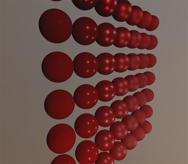
As the ambient light comes from all directions within the hemisphere oriented around the normal N, there’s no single halfway vector to determine the Fresnel response. To still simulate Fresnel, we calculate the Fresnel from the angle between the normal and view vector. However, earlier we used the micro-surface halfway vector, influenced by the roughness of the surface, as input to the Fresnel equation. As we currently don’t take roughness into account, the surface’s reflective ratio will always end up relatively high. Indirect light follows the same properties of direct light so we expect rougher surfaces to reflect less strongly on the surface edges. Because of this, the indirect Fresnel reflection strength looks off on rough non-metal surfaces (slightly exaggerated for demonstration purposes):

由于环境光来自以法线 N 为中心的半球内所有方向，不存在单一的半程向量来确定菲涅尔响应。为了仍能模拟菲涅尔效应，我们改为通过法线与视线向量的夹角来计算菲涅尔。然而，之前我们使用了受表面粗糙度影响的微表面半程向量作为菲涅尔方程的输入。但在当前的间接光照计算中，我们尚未考虑粗糙度的影响，这会导致表面的反射率在边缘区域始终偏高。间接光与直接光具有相同物理属性，理论上粗糙表面在边缘应拥有更弱的反射。因此，在粗糙的非金属表面上，间接菲涅尔反射强度会呈现失真现象（下图为刻意放大效果以作演示）：

We can alleviate the issue by injecting a roughness term in the Fresnel-Schlick equation as described by Sébastien Lagarde:

我们可以通过在菲涅尔-施利克方程中引入粗糙度项来缓解这个问题，如 Sébastien Lagarde 所述：

vec3 fresnelSchlickRoughness(float cosTheta, vec3 F0, float roughness)
{
    return F0 + (max(vec3(1.0 - roughness), F0) - F0) * pow(clamp(1.0 - cosTheta, 0.0, 1.0), 5.0);
}   

By taking account of the surface’s roughness when calculating the Fresnel response, the ambient code ends up as:

通过在计算菲涅尔响应时考虑表面粗糙度，环境光照部分的代码最终如下：

vec3 kS = fresnelSchlickRoughness(max(dot(N, V), 0.0), F0, roughness); 
vec3 kD = 1.0 - kS;
vec3 irradiance = texture(irradianceMap, N).rgb;
vec3 diffuse    = irradiance * albedo;
vec3 ambient    = (kD * diffuse) * ao; 

As you can see, the actual image based lighting computation is quite simple and only requires a single cubemap texture lookup; most of the work is in pre-computing or convoluting the irradiance map.

如你所见，基于图像的光照实际运行时计算代码非常简单，仅需查找采样一次立方体贴图纹理即可获得辐照度参数；绝大部分工作在于前期的预计算阶段，包括辐照度图的生成和卷积处理。

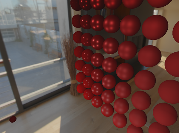
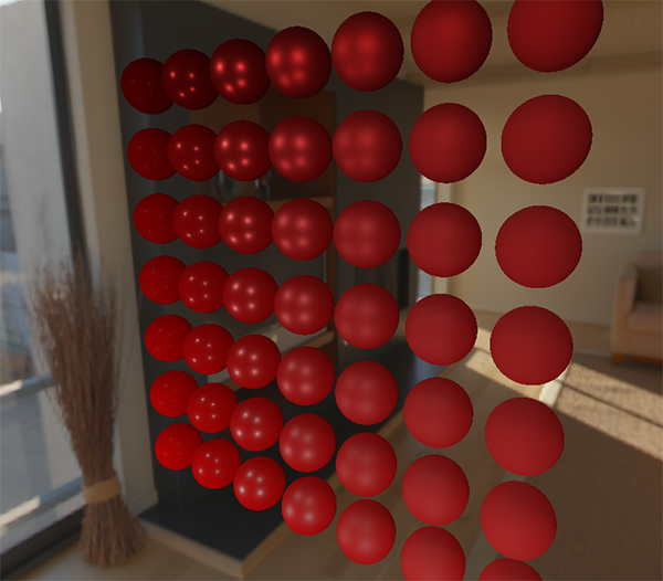
If we take the initial scene from the PBR lighting chapter, where each sphere has a vertically increasing metallic and a horizontally increasing roughness value, and add the diffuse image based lighting it’ll look a bit like this:

如果我们沿用 PBR 光照章节中的初始场景（每个球体的金属度沿垂直方向递增，粗糙度沿水平方向递增），并添加基于漫反射图像的光照，效果大致如下：

It still looks a bit weird as the more metallic spheres require some form of reflection to properly start looking like metallic surfaces (as metallic surfaces don’t reflect diffuse light) which at the moment are only (barely) coming from the point light sources. Nevertheless, you can already tell the spheres do feel more in place within the environment (especially if you switch between environment maps) as the surface response reacts accordingly to the environment’s ambient lighting.

现在看着还有一点怪异，因为金属质感球体更加依赖某种形式的反射（镜面反射）才能正确呈现金属表面特性（金属表面不会反射漫反射光），而目前只有点光源提供微弱反射。尽管如此，我们已能观察到球体与环境更协调的融合（切换不同环境贴图时尤为明显），其表面响应能准确反映环境光照特性。

You can find the complete source code of the discussed topics here. In the next chapter we’ll add the indirect specular part of the reflectance integral at which point we’re really going to see the power of PBR.

您可在此处获取相关主题的完整源码。在后续章节中，我们将加入反射积分的镜面反射分量——届时才能真正展现出基于物理渲染（PBR）的技术魅力。

References

• IBL Diffuse irradiance - LearnOpenGL