PBR --- Lighting

在本章中，我们将专注于把之前讨论的理论转化为实际的渲染器实现。

发表于 2024/06/17 更新于 2025/06/01

作者 LvXiao

38 分钟阅读

PBR --- Lighting

Introduction

In the previous chapter we laid the foundation for getting a realistic physically based renderer off the ground. In this chapter we’ll focus on translating the previously discussed theory into an actual renderer that uses direct (or analytic) light sources: think of point lights, directional lights, and/or spotlights.

在前面的章节中，我们为实现真实的基于物理的渲染器奠定了理论基础。在本章中，我们将专注于把之前讨论的理论转化为实际的渲染器实现，该渲染器将使用直接（或可解析）光源，例如点光源、方向光和或聚光灯。

Let’s start by re-visiting the final reflectance equation from the previous chapter:

让我们重新回顾前一章的最终反射方程，以此开始：

\[L_o{\small(p,\omega_o)} = \int\limits_{\Omega} \big( k_d\frac{c}{\pi} + \frac{DFG}{4 \big( \omega_o \cdot n \big) \big( \omega_i \cdot n \big)} \big) L_i{\small(p,\omega_i)} \big( n \cdot \omega_i \big) d\omega_i\]

We now know mostly what’s going on, but what still remained a big unknown is how exactly we’re going to represent irradiance, the total radiance $L$, of the scene. We know that radiance $L$ (as interpreted in computer graphics land) measures the radiant flux $\phi$ or light energy of a light source over a given solid angle $\omega$. In our case we assumed the solid angle $\omega$ to be infinitely small in which case radiance measures the flux of a light source over a single light ray or direction vector.

现在我们大致了解了整体情况，但仍有一个最大的未知数：我们究竟该如何表示场景的辐照度，即总的辐射率 $L$。我们知道，辐射率 $L$（如在计算机图形学领域中的定义）用于度量光源在给定立体角 $\omega$ 内的辐射通量 $\phi$（即光能）。在我们的讨论中，假设立体角 $\omega$ 无限小，此时辐射率表示光源在单一光线（或方向向量）上的通量。

Given this knowledge, how do we translate this into some of the lighting knowledge we’ve accumulated from previous chapters? Well, imagine we have a single point light (a light source that shines equally bright in all directions) with a radiant flux of (23.47, 21.31, 20.79) as translated to an RGB triplet. The radiant intensity of this light source equals its radiant flux at all outgoing direction rays. However, when shading a specific point $p$ on a surface, of all possible incoming light directions over its hemisphere $\Omega$, only one incoming direction vector $w_i$ directly comes from the point light source. As we only have a single light source in our scene, assumed to be a single point in space, all other possible incoming light directions have zero radiance observed over the surface point $p$:

基于这些知识，我们如何将其与前几章积累的光照知识联系起来呢？试想我们有一个单点光源（即在所有方向上发光强度均匀的光源），其辐射通量转换为 RGB 三元组后为 (23.47, 21.31, 20.79) 。该光源的辐射强度在所有出射方向光线上均等于其辐射通量。然而，当对表面上的特定点 $p$ 进行着色时，在其半球面 $\Omega$ 内的所有可能入射光方向中，只有一个入射方向向量 $w_i$ 直接来自点光源。由于场景中只有一个光源（假设为空间中的一个单一点），因此在表面点 $p$ 处观察到的所有其他可能入射光方向的辐射率均为零：

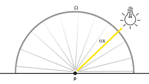对于未衰减的点光源，其在点 p 处的辐射率仅在无限小立体角 Wi（或光方向向量 Wi）上呈现非零值

If at first, we assume that light attenuation (dimming of light over distance) does not affect the point light source, the radiance of the incoming light ray is the same regardless of where we position the light (excluding scaling the radiance by the incident angle $\cos \theta$). This, because the point light has the same radiant intensity regardless of the angle we look at it, effectively modeling its radiant intensity as its radiant flux: a constant vector (23.47, 21.31, 20.79).

首先假设点光源不受光衰减（光线随距离的衰减）影响，那么入射光线的辐射率无论光源位置如何均保持不变（除了通过入射角 $\cos \theta$ 对辐射率进行缩放）。这是因为点光源在任何观察角度下均具有相同的辐射强度，从而有效地将其辐射强度模型化为辐射通量：一个恒定向量(23.47, 21.31, 20.79)。

However, radiance also takes a position $p$ as input and as any realistic point light source takes light attenuation into account, the radiant intensity of the point light source is scaled by some measure of the distance between point $p$ and the light source. Then, as extracted from the original radiance equation, the result is scaled by the dot product between the surface normal $n$ and the incoming light direction $w_i$.

然而，辐射率还将位置 $p$ 作为输入，并且任何真实的点光源都存在光衰减，因此点光源的辐射强度需按点 $p$ 与光源之间距离的某种度量进行缩放。然后，从原始辐射率方程中导出的结果需通过表面法线 $n$ 与入射光方向 $w_i$ 的点积进行缩放。

To put this in more practical terms: in the case of a direct point light the radiance function $L$ measures the light color, attenuated over its distance to $p$ and scaled by $n \cdot w_i$, but only over the single light ray $w_i$ that hits $p$ which equals the light’s direction vector from $p$. In code this translates to:

用更实际的术语来讲就是：在直接点光源的情况下，辐射率函数 $L$ 用于度量光的颜色，该颜色按其到 $p$ 的距离衰减，并通过 $n \cdot w_i$ 缩放，但仅在照射到 $p$ 的单条光线 $w_i$（该光线等于从 $p$ 指向光源的方向向量）上有效。在代码中，这可转化为：

  
vec3  lightColor  = vec3(23.47, 21.31, 20.79);
vec3  wi          = normalize(lightPos - fragPos);
float cosTheta    = max(dot(N, Wi), 0.0);
float attenuation = calculateAttenuation(fragPos, lightPos);
vec3  radiance    = lightColor * attenuation * cosTheta;

Aside from the different terminology, this piece of code should be awfully familiar to you: this is exactly how we’ve been doing diffuse lighting so far. When it comes to direct lighting, radiance is calculated similarly to how we’ve calculated lighting before as only a single light direction vector contributes to the surface’s radiance.

除了术语不同外，这段代码对你来说应该非常熟悉：这正是我们到目前为止计算漫反射光照的方式。在处理直接光照时，辐射率的计算方式与我们之前计算光照的方式类似，因为只有单个光线方向向量会对表面的辐射率产生影响。

Note that this assumption holds as point lights are infinitely small and only a single point in space. If we were to model a light that has area or volume, its radiance would be non-zero in more than one incoming light direction.

请注意，这一假设成立的前提是点光源无限小且为空间中的单个点。如果我们要建模一个具有面积或体积的光源，其辐射率将在多个入射光方向上为非零值。

For other types of light sources originating from a single point we calculate radiance similarly. For instance, a directional light source has a constant $w_i$ without an attenuation factor. And a spotlight would not have a constant radiant intensity, but one that is scaled by the forward direction vector of the spotlight.

对于其他源自单点的光源类型，我们以类似方式计算辐射率。例如，方向光源具有恒定的 $w_i$ 且无衰减因子；聚光灯的辐射强度则不是恒定的，而是按聚光灯的前向方向向量缩放。

This also brings us back to the integral $\int$ over the surface’s hemisphere $\Omega$. As we know beforehand the single locations of all the contributing light sources while shading a single surface point, it is not required to try and solve the integral. We can directly take the (known) number of light sources and calculate their total irradiance, given that each light source has only a single light direction that influences the surface’s radiance. This makes PBR on direct light sources relatively simple as we effectively only have to loop over the contributing light sources. When we later take environment lighting into account in the IBL chapters we do have to take the integral into account as light can come from any direction.

这也让我们回到对表面半球面 $\Omega$ 的积分 $\int$。由于在对单个表面点着色时，我们预先知道所有产生贡献的光源的位置，因此无需尝试求解积分。考虑到每个光源仅有一个影响表面辐射率的光线方向，我们可以直接计算已知数量光源的总辐照度。这使得基于直接光源的 PBR 相对简单，因为我们实际上只需遍历有贡献的光源。在后续关于IBL的章节中考虑环境光照时，我们必须考虑积分，因为光线可能来自任意方向。

A PBR surface model

Let’s start by writing a fragment shader that implements the previously described PBR models. First, we need to take the relevant PBR inputs required for shading the surface:

下面我们来编写一个实现此前描述的 PBR 模型的片段着色器。首先，我们需要获取着色表面所需的相关 PBR 输入：

  
#version 330 core
out vec4 FragColor;
in vec2 TexCoords;
in vec3 WorldPos;
in vec3 Normal;
  
uniform vec3 camPos;
  
uniform vec3  albedo;
uniform float metallic;
uniform float roughness;
uniform float ao;

We take the standard inputs as calculated from a generic vertex shader and a set of constant material properties over the surface of the object.

我们取从通用顶点着色器计算得到的标准输入，以及物体表面的一组恒定材质属性。

Then at the start of the fragment shader we do the usual calculations required for any lighting algorithm:

然后在片段着色器的起始部分，进行任何光照算法都需要的常规计算：

  
void main()
{
    vec3 N = normalize(Normal); 
    vec3 V = normalize(camPos - WorldPos);
    [...]
}

Direct lighting

In this chapter’s example demo we have a total of 4 point lights that together represent the scene’s irradiance. To satisfy the reflectance equation we loop over each light source, calculate its individual radiance and sum its contribution scaled by the BRDF and the light’s incident angle. We can think of the loop as solving the integral $\int$ over $\Omega$ for direct light sources. First, we calculate the relevant per-light variables:

在本章的示例演示中，我们总共有 4 个点光源，它们共同表示场景的辐照度。为了满足反射方程，我们遍历每个光源，计算其各自的辐射率，并将其贡献值按双向反射分布函数（BRDF）和光线入射角进行缩放后求和。我们可以将这个循环视为对直接光源在立体角 $\Omega$ 上求解积分 $\int$。首先，我们计算每个光源的相关变量：

  
vec3 Lo = vec3(0.0);
for(int i = 0; i < 4; ++i) 
{
    vec3 L = normalize(lightPositions[i] - WorldPos);
    vec3 H = normalize(V + L);
  
    float distance    = length(lightPositions[i] - WorldPos);
    float attenuation = 1.0 / (distance * distance);
    vec3 radiance     = lightColors[i] * attenuation; 
    [...]  

As we calculate lighting in linear space (we’ll gamma correct at the end of the shader) we attenuate the light sources by the more physically correct inverse-square law.

由于我们在线性空间中计算光照（会在着色器的最后进行伽马校正），所以会采用更符合物理规律的平方反比定律来衰减光源。

While physically correct, you may still want to use the constant-linear-quadratic attenuation equation that (while not physically correct) can offer you significantly more control over the light’s energy falloff.

尽管使用平方反比定律在物理上是正确的，但你可能仍想使用恒定-线性-二次衰减方程。虽然该方程在物理上并不准确，但它能让你更灵活地控制光的能量衰减。

Then, for each light we want to calculate the full Cook-Torrance specular BRDF term:

接下来，对于每个光源，我们需要计算完整的 Cook-Torrance 镜面 BRDF 项：

\[\frac{DFG}{4 \big( \omega_o \cdot n \big) \big( \omega_i \cdot n \big)}\]

The first thing we want to do is calculate the ratio between specular and diffuse reflection, or how much the surface reflects light versus how much it refracts light. We know from the previous chapter that the Fresnel equation calculates just that (note the clamp here to prevent black spots):

我们要做的第一件事是计算镜面反射与漫反射的比率，即表面反射光与折射光的比例。从前一章可知，菲涅尔方程正是用于计算这一比率的（注意此处的钳制是为了避免出现黑点）：

  
vec3 fresnelSchlick(float cosTheta, vec3 F0)
{
    return F0 + (1.0 - F0) * pow(clamp(1.0 - cosTheta, 0.0, 1.0), 5.0);
}  

The Fresnel-Schlick approximation expects a F0 parameter which is known as the surface reflection at zero incidence or how much the surface reflects if looking directly at the surface. The F0 varies per material and is tinted on metals as we find in large material databases. In the PBR metallic workflow we make the simplifying assumption that most dielectric surfaces look visually correct with a constant F0 of 0.04, while we do specify F0 for metallic surfaces as then given by the albedo value. This translates to code as follows:

菲涅尔-施利克近似需要一个 F0 参数，即零入射角下的表面反射率，也就是当视线垂直于表面时的反射率。F0 的值因材质而异，在金属表面上还会呈现颜色，这一点可在大型材质数据库中查到。在基于物理的金属工作流中，我们做了一个简化假设：大多数电介质表面使用固定的 F0 = 0.04 就能在视觉上获得正确效果，而金属表面的 F0 则直接由反照率（albedo）值确定。这一逻辑对应的代码如下：

  
vec3 F0 = vec3(0.04); 
F0      = mix(F0, albedo, metallic);
vec3 F  = fresnelSchlick(max(dot(H, V), 0.0), F0);

As you can see, for non-metallic surfaces F0 is always 0.04. For metallic surfaces, we vary F0 by linearly interpolating between the original F0 and the albedo value given the metallic property.

如你所见，对于非金属表面，F0 始终为 0.04。对于金属表面，我们根据 metallic 属性，通过在原始 F0 值与反照率值之间进行线性插值来调整 F0。

Given $F$, the remaining terms to calculate are the normal distribution function $D$ and the geometry function $G$.

给定 $F$ 后，剩下需要计算的项是法线分布函数 $D$ 和几何函数 $G$。

In a direct PBR lighting shader their code equivalents are:

在直接光照的PBR着色器中，它们对应的代码实现如下：

  
float DistributionGGX(vec3 N, vec3 H, float roughness)
{
    float a      = roughness*roughness;
    float a2     = a*a;
    float NdotH  = max(dot(N, H), 0.0);
    float NdotH2 = NdotH*NdotH;
	
    float num   = a2;
    float denom = (NdotH2 * (a2 - 1.0) + 1.0);
    denom = PI * denom * denom;
	
    return num / denom;
}

float GeometrySchlickGGX(float NdotV, float roughness)
{
    float r = (roughness + 1.0);
    float k = (r*r) / 8.0;

    float num   = NdotV;
    float denom = NdotV * (1.0 - k) + k;
	
    return num / denom;
}
float GeometrySmith(vec3 N, vec3 V, vec3 L, float roughness)
{
    float NdotV = max(dot(N, V), 0.0);
    float NdotL = max(dot(N, L), 0.0);
    float ggx2  = GeometrySchlickGGX(NdotV, roughness);
    float ggx1  = GeometrySchlickGGX(NdotL, roughness);
	
    return ggx1 * ggx2;
}

What’s important to note here is that in contrast to the theory chapter, we pass the roughness parameter directly to these functions; this way we can make some term-specific modifications to the original roughness value. Based on observations by Disney and adopted by Epic Games, the lighting looks more correct squaring the roughness in both the geometry and normal distribution function.

这里需要重点注意的是，与 PBR Theory 章节不同，我们将粗糙度参数直接传递给这些函数；通过这种方式，我们可以对原始粗糙度值进行某些特定于项的修改。基于 Disney 的观察并被 Epic Games 采用的做法是，在几何函数和正态分布函数中对粗糙度进行平方处理时，光照效果看起来更为正确。

With both functions defined, calculating the NDF and the G term in the reflectance loop is straightforward:

定义了这两个函数之后，在反射循环体中计算法线分布函数(NDF)和几何遮蔽函数(G)这两项就很简单了：

  
float NDF = DistributionGGX(N, H, roughness);       
float G   = GeometrySmith(N, V, L, roughness); 

This gives us enough to calculate the Cook-Torrance BRDF:

这使我们有足够的条件来计算 Cook-Torrance 双向反射分布函数(BRDF)：

  
vec3 numerator    = NDF * G * F;
float denominator = 4.0 * max(dot(N, V), 0.0) * max(dot(N, L), 0.0)  + 0.0001;
vec3 specular     = numerator / denominator; 

Note that we add 0.0001 to the denominator to prevent a divide by zero in case any dot product ends up 0.0.

请注意，我们在分母中添加了 0.0001，以防止在任何点积结果为 0.0 的情况下出现除以零的错误。

Now we can finally calculate each light’s contribution to the reflectance equation. As the Fresnel value directly corresponds to $k_S$ we can use $F$ to denote the specular contribution of any light that hits the surface. From $k_S$ we can then calculate the ratio of refraction $k_D$:

现在我们终于可以计算每个光源对反射方程的贡献了。由于菲涅尔值直接对应于 $k_S$，我们可以使用 $F$ 来表示任何照射到表面的光线的镜面反射贡献。然后，从 $k_S$ 我们可以计算折射比例 $k_D$：

  
vec3 kS = F;
vec3 kD = vec3(1.0) - kS;
  
kD *= 1.0 - metallic;	

Seeing as kS represents the energy of light that gets reflected, the remaining ratio of light energy is the light that gets refracted which we store as kD. Furthermore, because metallic surfaces don’t refract light and thus have no diffuse reflections we enforce this property by nullifying kD if the surface is metallic. This gives us the final data we need to calculate each light’s outgoing reflectance value:

鉴于 kS 表示被反射的光线能量，剩余的光线能量比例就是被折射的光线，我们将其存储为 kD。此外，由于金属表面不会折射光线，因此没有漫反射，所以如果表面是金属材质，我们会将 kD 设为零来强化这一特性。这就为我们提供了计算每个光源的出射反射值所需的最终数据：

  
    const float PI = 3.14159265359;
  
    float NdotL = max(dot(N, L), 0.0);        
    Lo += (kD * albedo / PI + specular) * radiance * NdotL;
}

The resulting Lo value, or the outgoing radiance, is effectively the result of the reflectance equation’s integral $\int$ over $\Omega$. We don’t really have to try and solve the integral for all possible incoming light directions as we know exactly the 4 incoming light directions that can influence the fragment. Because of this, we can directly loop over these incoming light directions e.g. the number of lights in the scene.

得到的 Lo 值，即出射辐射率，实际上就是反射方程在立体角 $\Omega$ 上的积分 $\int$ 结果。由于我们明确知道可能影响该片段的 4 个入射光线方向，所以无需尝试对所有可能的入射光线方向求解积分。因此，已知场景中的光源数量，我们可以直接遍历这些入射光线方向。

What’s left is to add an (improvised) ambient term to the direct lighting result Lo and we have the final lit color of the fragment:

剩下要做的就是将一个（临时添加的）环境光照项添加到直接光照结果 Lo 中，这样我们就得到了该片段的最终光照颜色：

  
vec3 ambient = vec3(0.03) * albedo * ao;
vec3 color   = ambient + Lo;

Linear and HDR rendering

So far we’ve assumed all our calculations to be in linear color space and to account for this we need to gamma correct at the end of the shader. Calculating lighting in linear space is incredibly important as PBR requires all inputs to be linear. Not taking this into account will result in incorrect lighting. Additionally, we want light inputs to be close to their physical equivalents such that their radiance or color values can vary wildly over a high spectrum of values. As a result, Lo can rapidly grow really high which then gets clamped between 0.0 and 1.0 due to the default low dynamic range (LDR) output. We fix this by taking Lo and tone or exposure map the high dynamic range (HDR) value correctly to LDR before gamma correction:

到目前为止，我们一直假设所有计算都在线性色彩空间中进行，因此需要在着色器的最后进行伽马校正。在线性空间中计算光照非常重要，因为 PBR 要求所有输入都是线性的。不考虑这一点将导致光照计算错误。此外，我们希望光照输入尽可能接近其物理等效值，这样它们的辐射率或颜色值可以在很宽的范围内变化。因此，Lo 值可能会迅速变得非常高，但由于默认的低动态范围（LDR）输出，这些值会被限制在 0.0 到 1.0 之间。我们通过对 Lo 进行色调映射或曝光映射，将高动态范围（HDR）值正确转换为低动态范围（LDR）值，然后再进行伽马校正来解决这个问题：

  
color = color / (color + vec3(1.0));
color = pow(color, vec3(1.0/2.2)); 

Here we tone map the HDR color using the Reinhard operator, preserving the high dynamic range of a possibly highly varying irradiance, after which we gamma correct the color. We don’t have a separate framebuffer or post-processing stage so we can directly apply both the tone mapping and gamma correction step at the end of the forward fragment shader.

在这里，我们使用 Reinhard 算子对 HDR 颜色进行色调映射，以保留可能高度变化的辐照度的高动态范围，然后对颜色进行伽马校正。由于我们没有单独的帧缓冲或后处理阶段，因此可以在前向片段着色器的末尾直接应用色调映射和伽马校正步骤。

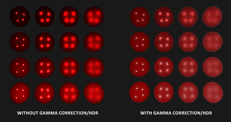
Taking both linear color space and high dynamic range into account is incredibly important in a PBR pipeline. Without these it’s impossible to properly capture the high and low details of varying light intensities and your calculations end up incorrect and thus visually unpleasing.

在 PBR 管线中，同时考虑线性色彩空间和高动态范围（HDR）极为重要。若不考虑这些因素，将无法正确捕捉不同光照强度的高低细节，导致计算结果错误，进而在视觉效果上令人不满意。

Full direct lighting PBR shader

All that’s left now is to pass the final tone mapped and gamma corrected color to the fragment shader’s output channel and we have ourselves a direct PBR lighting shader. For completeness’ sake, the complete main function is listed below:

现在剩下的就是将最终经过色调映射和伽马校正的颜色传递给片段着色器的输出通道，这样我们就实现了一个直接的 PBR 光照着色器。为了完整性，下面列出完整的 main 函数：

  
#version 330 core
out vec4 FragColor;
in vec2 TexCoords;
in vec3 WorldPos;
in vec3 Normal;

// material parameters
uniform vec3  albedo;
uniform float metallic;
uniform float roughness;
uniform float ao;

// lights
uniform vec3 lightPositions[4];
uniform vec3 lightColors[4];

uniform vec3 camPos;

const float PI = 3.14159265359;
  
float DistributionGGX(vec3 N, vec3 H, float roughness);
float GeometrySchlickGGX(float NdotV, float roughness);
float GeometrySmith(vec3 N, vec3 V, vec3 L, float roughness);
vec3 fresnelSchlick(float cosTheta, vec3 F0);

void main()
{		
    vec3 N = normalize(Normal);
    vec3 V = normalize(camPos - WorldPos);

    vec3 F0 = vec3(0.04); 
    F0 = mix(F0, albedo, metallic);
	           
    // reflectance equation
    vec3 Lo = vec3(0.0);
    for(int i = 0; i < 4; ++i) 
    {
        // calculate per-light radiance
        vec3 L = normalize(lightPositions[i] - WorldPos);
        vec3 H = normalize(V + L);
        float distance    = length(lightPositions[i] - WorldPos);
        float attenuation = 1.0 / (distance * distance);
        vec3 radiance     = lightColors[i] * attenuation;        
        
        // cook-torrance brdf
        float NDF = DistributionGGX(N, H, roughness);        
        float G   = GeometrySmith(N, V, L, roughness);      
        vec3 F    = fresnelSchlick(max(dot(H, V), 0.0), F0);       
        
        vec3 kS = F;
        vec3 kD = vec3(1.0) - kS;
        kD *= 1.0 - metallic;	  
        
        vec3 numerator    = NDF * G * F;
        float denominator = 4.0 * max(dot(N, V), 0.0) * max(dot(N, L), 0.0) + 0.0001;
        vec3 specular     = numerator / denominator;  
            
        // add to outgoing radiance Lo
        float NdotL = max(dot(N, L), 0.0);                
        Lo += (kD * albedo / PI + specular) * radiance * NdotL; 
    }   
  
    vec3 ambient = vec3(0.03) * albedo * ao;
    vec3 color = ambient + Lo;
	
    color = color / (color + vec3(1.0));
    color = pow(color, vec3(1.0/2.2));  
   
    FragColor = vec4(color, 1.0);
}  

Hopefully, with the theory from the previous chapter and the knowledge of the reflectance equation this shader shouldn’t be as daunting anymore. If we take this shader, 4 point lights, and quite a few spheres where we vary both their metallic and roughness values on their vertical and horizontal axis respectively, we’d get something like this:

希望通过上一章的理论和反射方程的知识，这个着色器不再那么令人生畏。如果我们使用这个着色器，设定 4 个点光源，安排一组金属度和粗糙度可变的球体，分别在垂直和水平方向上改变球体的金属度和粗糙度值，我们会得到这样的效果：

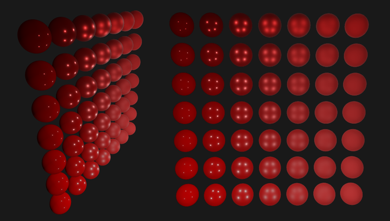
From bottom to top the metallic value ranges from 0.0 to 1.0, with roughness increasing left to right from 0.0 to 1.0. You can see that by only changing these two simple to understand parameters we can already display a wide array of different materials.

从下到上金属度值从 0.0 到 1.0，从左到右粗糙度从 0.0 到 1.0 递增。可以看到，仅通过改变这两个易于理解的参数，我们就已经能够呈现各种各样的不同材质。

You can find the full source code of the demo here.

你可以在此处找到该示例的完整源代码。

Textured PBR

Extending the system to now accept its surface parameters as textures instead of uniform values gives us per-fragment control over the surface material’s properties:

扩展系统，让其接受纹理作为表面参数输入，以取代之前的 unifrom 值，这使得我们能够对每个片段的表面材质属性都进行控制：

  
[...]
uniform sampler2D albedoMap;
uniform sampler2D normalMap;
uniform sampler2D metallicMap;
uniform sampler2D roughnessMap;
uniform sampler2D aoMap;
  
void main()
{
    vec3 albedo     = pow(texture(albedoMap, TexCoords).rgb, 2.2);
    vec3 normal     = getNormalFromNormalMap();
    float metallic  = texture(metallicMap, TexCoords).r;
    float roughness = texture(roughnessMap, TexCoords).r;
    float ao        = texture(aoMap, TexCoords).r;
    [...]
}

Note that the albedo textures that come from artists are generally authored in sRGB space which is why we first convert them to linear space before using albedo in our lighting calculations. Based on the system artists use to generate ambient occlusion maps you may also have to convert these from sRGB to linear space as well. Metallic and roughness maps are almost always authored in linear space.

请注意，艺术家创建的反照率纹理通常是在 sRGB 空间中制作的，这就是为什么我们在光照计算中使用反照率之前首先要将它们转换为线性空间的原因。对于环境光遮蔽贴图，根据艺术家用于生成其的系统，你可能需要将这些环境光遮蔽贴图也从 sRGB 转换为线性空间。金属度和粗糙度贴图几乎总是在线性空间中制作的，不需要转换处理。

Replacing the material properties of the previous set of spheres with textures, already shows a major visual improvement over the previous lighting algorithms we’ve used:

用纹理替换之前那一组球体的材质属性，相比于我们之前使用的光照算法，已经可以看出有了重大的视觉效果提升：

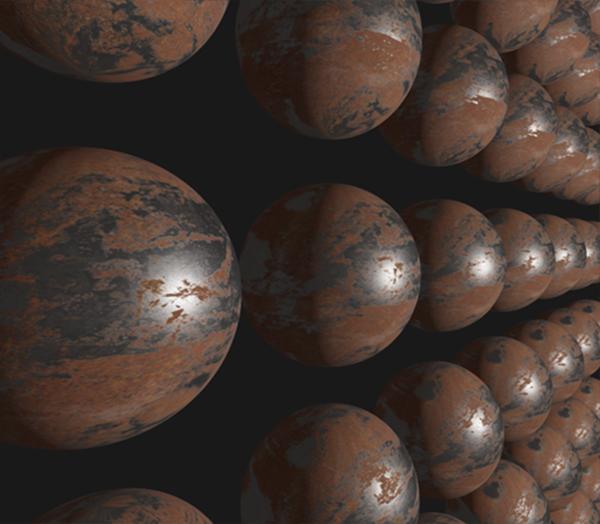
You can find the full source code of the textured demo here and the texture set used here (with a white ao map). Keep in mind that metallic surfaces tend to look too dark in direct lighting environments as they don’t have diffuse reflectance. They do look more correct when taking the environment’s specular ambient lighting into account, which is what we’ll focus on in the next chapters.

你可以在此处找到带纹理的示例程序的完整源代码，以及在此处找到所用的纹理集（带有白色环境光遮蔽贴图）。请记住，因为金属表面没有漫反射，它们在直接光照环境中往往看起来会很暗。当考虑环境的镜面环境光照时，它们看起来会更自然，这正是我们在下一章要关注的内容。

While not as visually impressive as some of the PBR render demos you find out there, given that we don’t yet have image based lighting built in, the system we have now is still a physically based renderer, and even without IBL you’ll see your lighting look a lot more realistic.

虽然由于尚未集成基于图像的光照，我们的系统还在视觉上没那么震撼，不如你在其他地方看到的一些 PBR 渲染示例，但我们现在拥有的仍然是一个基于物理的渲染器，即使没有 IBL，你也会看到你的光照效果比之前更加真实。

References

PBR Lighting - LearnOpenGL

Computer Grahics, LearnOpenGL, PBR

本文由作者按照 CC BY 4.0 进行授权